Clinical Programming in R

Workshop for Ukraine

Edoardo Mancini - 17th September 2026

About Me & This Workshop

I am a Senior Data Scientist working at Roche in the UK. My work involves leading statistical programming activities in early and late-stage clinical trials. I am also a passionate advocate for R and Open Source, and am able to pursue these interests in my current role as maintainer for the {admiral} R package.

Outside of work, I enjoy playing chess♟️, reading📖, and running🏃.

Donations for sign-ups to this workshop (both live and in future) will be used to support the Ukraine War Effort 🙏.

Welcome!

What we’ll do today:

Understand the clinical trial data flow
Derive analysis variables on real-format study data
Build a publication-quality visualisation

Workshop materials

For slides, template and data, please see the workshop GitHub repo here.

Please install the following packages in R while we go through the background section:

install.packages("pharmaversesdtm") # test data
install.packages("admiral") # tools for ADaM programming
install.packages("ggplot2") # plots

You may also want to clone the GitHub repository to your local session, or at least have it open in a browser tab to follow the slides and access the template code.

Agenda

We have a lot to cover:

Time	Topic
0:00	Welcome and Intro
0:05	Background: The Clinical Trial Data Journey
0:25	Exercise Setup, Test data and the Packages we’ll be Using
0:30	Exercise 1 — `ADSL` Derivations
1:00	Exercise 2 — `ADVS` Derivations
1:30	Exercise 3 — A Simple Plot
1:55	Wrap-up and Next Steps

The background section will give you enough context to be able to do the three exercises, hopefully without overloading you with too much information!

Background: The Clinical Trial Data Journey

The Clinical Trial Data Journey

The journey of a data point from a patient to a regulator’s report is long and complex! It can loosely be categorised into four stages:

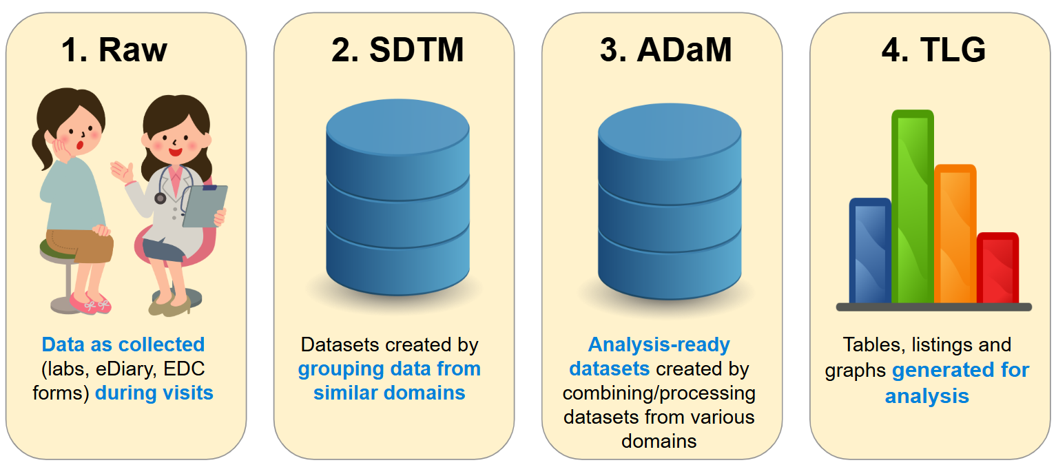
Let’s go through these stages one by one…

1. Raw Data — Where it all begins!

Data enters a clinical trial from many sources:

eDiary / CRF (case report form): clinician- or patient-reported data (e.g. adverse events, concomitant medications, etc)
Central labs: blood tests, urinalysis
Wearables / devices: ECG, vital signs monitors

Raw data is messy!

Different units, different date formats
Inconsistent coding (a “heart attack” might be “MI”, “myocardial infarction”, or “cardiac event”)
Missing or partial dates

So we process raw data into…

2. SDTM — Standardising the data

SDTM (Study Data Tabulation Model) groups similar, related data into domains. Here are some below.

Domain	Contents
`DM`	Demographics
`VS`	Vital Signs
`LB`	Laboratory
`AE`	Adverse Events
`EX`	Exposure (drug dosing)

E.g. the labs domain groups all the blood tests, urinalysis etc into one dataset.

Key features of SDTM

One row per observation, e.g.:
- In DM: one row per patient
- In LB: one row per patient per lab test per visit;
- In AE: one row per patient per adverse event
Standard variable names across all studies
Standardised units
Reported terms are coded where appropriate (e.g. “Heart attack”, “Cardiac arrest” → “Myocardial Infarction”).

🤔Open question: Can you think of any other domains?

Let’s see some examples…

SDTM in action: `DM` & `EX`

DM (Demographics) — one row per patient

USUBJID Unique Subject Identifier	AGE Age	RACE Race	COUNTRY Country	ARM Description of Planned Arm
01-701-1015	63	WHITE	USA	Placebo
01-701-1023	64	WHITE	USA	Placebo
01-701-1028	71	WHITE	USA	Xanomeline High Dose
01-701-1033	74	WHITE	USA	Xanomeline Low Dose
01-701-1034	77	WHITE	USA	Xanomeline High Dose
01-701-1047	85	WHITE	USA	Placebo
01-701-1057	59	WHITE	USA	Screen Failure
01-701-1097	68	WHITE	USA	Xanomeline Low Dose
01-701-1111	81	WHITE	USA	Xanomeline Low Dose
01-701-1115	84	WHITE	USA	Xanomeline Low Dose

EX (Drug Exposure) — one row per patient per dosing

USUBJID Unique Subject Identifier	EXTRT Name of Actual Treatment	VISIT Visit Name	EXSTDTC Start Date/Time of Treatment	EXDOSE Dose per Administration
01-701-1015	PLACEBO	BASELINE	2014-01-02	0
01-701-1015	PLACEBO	WEEK 2	2014-01-17	0
01-701-1015	PLACEBO	WEEK 24	2014-06-19	0
01-701-1023	PLACEBO	BASELINE	2012-08-05	0
01-701-1023	PLACEBO	WEEK 2	2012-08-28	0
01-701-1028	XANOMELINE	BASELINE	2013-07-19	54
01-701-1028	XANOMELINE	WEEK 2	2013-08-02	81
01-701-1028	XANOMELINE	WEEK 24	2014-01-07	54
01-701-1033	XANOMELINE	BASELINE	2014-03-18	54
01-701-1034	XANOMELINE	BASELINE	2014-07-01	54

SDTM in action: `AE` & `VS`

AE (Adverse Events) — one row per patient per adverse event

USUBJID Unique Subject Identifier	AEDECOD Dictionary-Derived Term	AESER Serious Event	AESEV Severity/ Intensity	AESTDTC Start Date/ Time of Adverse Event
01-701-1015	APPLICATION SITE ERYTHEMA	N	MILD	2014-01-03
01-701-1015	APPLICATION SITE PRURITUS	N	MILD	2014-01-03
01-701-1015	DIARRHOEA	N	MILD	2014-01-09
01-701-1023	ATRIOVENTRICULAR BLOCK SECOND DEGREE	N	MILD	2012-08-26
01-701-1023	ERYTHEMA	N	MILD	2012-08-07
01-701-1023	ERYTHEMA	N	MODERATE	2012-08-07
01-701-1023	ERYTHEMA	N	MILD	2012-08-07
01-701-1028	APPLICATION SITE ERYTHEMA	N	MILD	2013-07-21
01-701-1028	APPLICATION SITE PRURITUS	N	MILD	2013-08-08

VS (Vital Signs) — one row per patient per vital sign measurement

USUBJID Unique Subject Identifier	VSTESTCD Vital Signs Test Short Name	VSORRES Result or Finding in Original Units	VSORRESU Original Units	VISIT Visit Name
01-701-1015	HEIGHT	58.0	IN	SCREEN 1
01-701-1015	PULSE	62	BEATS/MIN	SCREEN 1
01-701-1015	PULSE	60	BEATS/MIN	SCREEN 2
01-701-1015	PULSE	59	BEATS/MIN	BASELINE
01-701-1015	PULSE	61	BEATS/MIN	WEEK 2
01-701-1015	PULSE	62	BEATS/MIN	WEEK 4
01-701-1015	PULSE	56	BEATS/MIN	WEEK 6
01-701-1015	PULSE	60	BEATS/MIN	WEEK 8
01-701-1015	PULSE	53	BEATS/MIN	WEEK 12
01-701-1015	PULSE	55	BEATS/MIN	WEEK 16
01-701-1015	PULSE	59	BEATS/MIN	WEEK 20
01-701-1015	PULSE	57	BEATS/MIN	WEEK 24
01-701-1015	PULSE	61	BEATS/MIN	WEEK 26
01-701-1023	HEIGHT	64.0	IN	SCREEN 1
01-701-1023	PULSE	78	BEATS/MIN	SCREEN 1
01-701-1023	PULSE	91	BEATS/MIN	SCREEN 2

But what if we want to combine data from different domains or compute new variables for analysis?

3. ADaM — Analysis-ready datasets

ADaM (Analysis Data Model) transforms and combines SDTM into datasets ready for statistical analysis.

The step from SDTM to ADaM can involve complex programming, as we are trying to set up the data to answer the questions about safety and efficacy that the clinical trial is posing, and this often involves combining domains.

A typical example

We may be interested in exploring whether patients are likely to have an adverse event after being exposed to the drug. So in ADAE (Adverse Events Analysis Dataset) we would compute the time since last dose for every adverse event - ready to then be used in a table/graph. This would need to use information from ADSL and/or EX.

Key features of ADaM

Analysis values and computation of change from baseline
Derived rows (e.g. deriving mean arterial pressure from systolic and diastolic BP)
Population flags (e.g. Safety population SAFFL, flagging all patients who have received a dose of study drug).

Today, we’ll start directly from the ADaM-building stage. For the first part of our exercises, we will be working with two ADaM datasets - ADSL (Subject level ADaM, derived from DM) and ADVS (Vital Signs ADaM, derived from VS).

But first, let’s see what some typical ADAMs (ADSL, ADVS and ADAE) might look like…

ADaM in action: `ADSL`

ADSL (Subject-Level Analysis Dataset) — one row per subject (derived from DM, DS, AE, etc.). Variables highlighted in yellow are derived.

USUBJID Unique Subject Identifier	AGE Age	SEX Sex	RACE Race	TRT01A Actual Treatment for Period 01	AGEGR1 Pooled Age Group 1	SAFFL Safety Population Flag	RANDDT Date of Randomization	TRTSDTM Datetime of First Exposure to Treatment	TRTEDTM Datetime of Last Exposure to Treatment	DTHDT Date of Death
01-701-1015	63	F	WHITE	Placebo	18-64	Y	2014-01-02	2014-01-02	2014-07-02 23:59:59	NA
01-701-1023	64	M	WHITE	Placebo	18-64	Y	2012-08-05	2012-08-05	2012-09-01 23:59:59	NA
01-701-1028	71	M	WHITE	Xanomeline High Dose	>64	Y	2013-07-19	2013-07-19	2014-01-14 23:59:59	NA
01-701-1033	74	M	WHITE	Xanomeline Low Dose	>64	Y	2014-03-18	2014-03-18	2014-03-31 23:59:59	NA
01-701-1034	77	F	WHITE	Xanomeline High Dose	>64	Y	2014-07-01	2014-07-01	2014-12-30 23:59:59	NA
01-701-1047	85	F	WHITE	Placebo	>64	Y	2013-02-12	2013-02-12	2013-03-09 23:59:59	NA
01-701-1057	59	F	WHITE	Screen Failure	18-64	N	NA	NA	NA	NA

ADaM in action: `ADAE`

ADAE (Adverse Events Analysis Dataset) — one row per patient per adverse event (derived from AE + ADSL + EX). Variables highlighted in purple come from ADSL. Variables highlighted in yellow are derived.

USUBJID Unique Subject Identifier	TRT01A Actual Treatment for Period 01	TRTSDTM Treatment Start Datetime	AEDECOD Dictionary-Derived Term	AESTDTC Start Date/Time of Adverse Event	AESER Serious Event	AESEV Severity/ Intensity	ASTDY Analysis Start Relative Day	TRTEMFL Treatment Emergent Flag	LDOSEDTM (Dummy) Last Dose Datetime
01-701-1015	Placebo	2014-01-02	APPLICATION SITE ERYTHEMA	2014-01-03	MILD	N	2	Y	2014-01-02 23:59:59
01-701-1015	Placebo	2014-01-02	APPLICATION SITE PRURITUS	2014-01-03	MILD	N	2	Y	2014-01-02 23:59:59
01-701-1015	Placebo	2014-01-02	DIARRHOEA	2014-01-09	MILD	N	8	Y	2014-01-08 23:59:59
01-701-1023	Placebo	2012-08-05	ERYTHEMA	2012-08-07	MODERATE	N	3	Y	2012-08-06 23:59:59
01-701-1023	Placebo	2012-08-05	ERYTHEMA	2012-08-07	MILD	N	3	Y	2012-08-06 23:59:59

🤔Open question: Can you think of any other information we may want to collect or derive about an adverse event?

ADaM in action: `ADVS`

ADVS (Vital Signs Analysis Dataset) — one row per patient per parameter per visit (derived from VS and ADSL). Records highlighted in yellow are derived.

USUBJID Unique Subject Identifier	TRT01A Actual Treatment for Period 01	PARAMCD Parameter Code	PARAM Parameter	DTYPE Derivation Type	AVISIT Analysis Visit	AVISITN Analysis Visit (N)	ABLFL Baseline Record Flag	AVAL Analysis Value	BASE Baseline Value	CHG Change from Baseline
01-701-1015	Placebo	DIABP	Diastolic Blood Pressure (mmHg)	NA	Baseline	0	Y	51	51	0
01-701-1015	Placebo	SYSBP	Systolic Blood Pressure (mmHg)	NA	Baseline	0	Y	121	121	0
01-701-1015	Placebo	MAP	Mean Arterial Pressure	DERIVED	Baseline	0	Y	86	86	0
01-701-1015	Placebo	DIABP	Diastolic Blood Pressure (mmHg)	NA	Week 2	2	NA	50	51	-1
01-701-1015	Placebo	SYSBP	Systolic Blood Pressure (mmHg)	NA	Week 2	2	NA	121	121	0
01-701-1015	Placebo	MAP	Mean Arterial Pressure	DERIVED	Week 2	2	NA	85.5	86	-0.5
01-701-1015	Placebo	DIABP	Diastolic Blood Pressure (mmHg)	NA	Week 4	4	NA	55	51	4
01-701-1015	Placebo	SYSBP	Systolic Blood Pressure (mmHg)	NA	Week 4	4	NA	137	121	16
01-701-1015	Placebo	MAP	Mean Arterial Pressure	DERIVED	Week 4	4	NA	96	86	10

And with these ADaMs, we can finally produce…

4. TLGs — Answering questions!

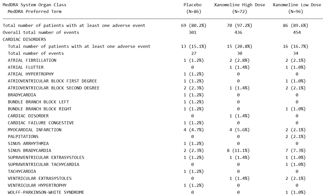
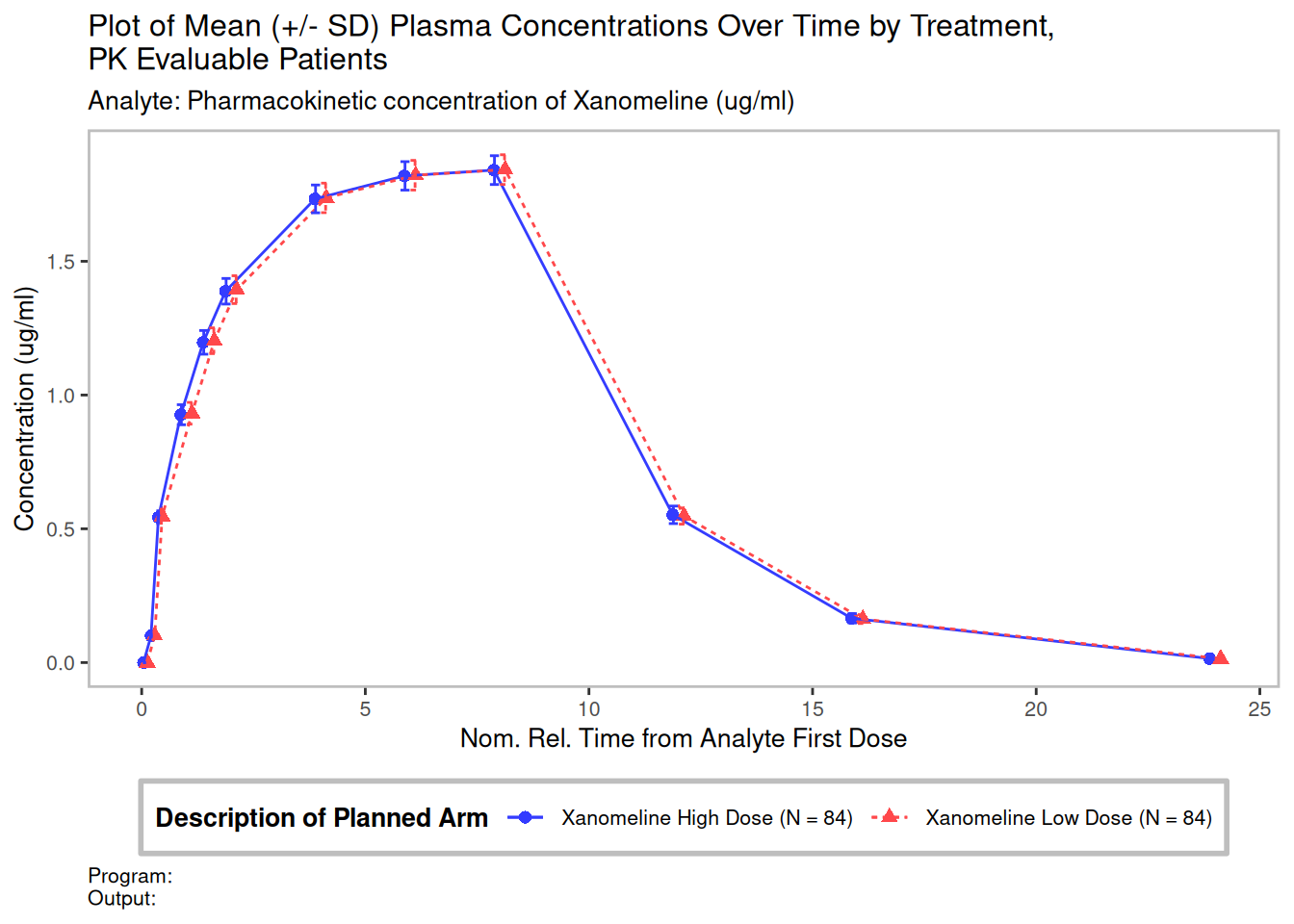
The final TLGs (tables, listings and graphs) that answer questions about the trial’s safety and efficacy. These are provided to regulators and used in publications.

In today’s workshop’s last exercise, we will focus on creating a vital signs plot.

But first, let’s see a typical table and plot for a clinical trial…

TLG Example: AE Table

TLG Example: Pharmacokinetic Plot

Exercise Setup, Test Data & Packages

Exercise Setup and Test Data

Welcome to the interactive part of the workshop! Here we will focus on:

Creating two ADaM datasets, ADSL (Subject-level) and ADVS (Vital Signs) - Exercises 1 and 2;
Creating a plot of Mean Arterial Pressure over time using these datasets - Exercise 3.

We will be using test data today. The source for the test data is the {pharmaversesdtm} package. This is the same test data that has been used for the examples in the background section.

Where does this data come from?

{pharmaversesdtm} is one of the package maintained by members of the pharmaverse, which is an Open-Source effort to set up a toolset for End-to-End clinical reporting in R. You can access the test datasets like so:

library(pharmaversesdtm)

# Demographics
pharmaversesdtm::dm

# Vital signs
pharmaversesdtm::vs

Luckily, you won’t have to create anything from scratch: the templates folder in the GitHub repo contains starting programs on which the exercises are based.

Packages

As well as the {tidyverse} suite of packages, today we will be using another pharmaverse package, {admiral}, to help us create our ADaM datasets.

library(admiral)

What’s the idea behind {admiral}

Core idea: {admiral} derive_*() functions can be chained together with {dplyr} functions in a series of blocks, each modifying a dataset in some way, e.g. adding variables or rows.

Take a look at the two blocks below:

adsl_start <- dm %>%
  ## Derive treatment arm variables
  mutate(TRT01P = ARM, TRT01A = ACTARM) %>%
  ## Derive treatment start datetime / date 
  derive_vars_merged(
    dataset_add = ex,
    by_vars = exprs(STUDYID, USUBJID),
    filter_add = (EXDOSE > 0 | (EXDOSE == 0 & str_detect(EXTRT, "PLACEBO"))) & !is.na(EXSTDTM),
    order = exprs(EXSTDTM, EXSEQ),
    mode = "first",       
    new_vars = exprs(TRTSDTM = EXSTDTM)
  )

Notice in particular the use of exprs() to pass column names, and by_vars to split the dataset into groups.

We’ll be using {ggplot2} for our plot… but you’re all probably familiar with that already!

Exercise 1: Working with `ADSL`

Let’s remind ourselves of what we can find in the ADSL dataset.

ADSL contains one row per patient - so the number of rows of the dataset is equal to the total number of patients in the trial.

Here are some of the key variables in the ADSL dataset:

Variable	Description
`USUBJID`	Unique subject identifier (i.e. an anonymous code that labels the patient)
`AGE`, `SEX`, `RACE`	Demographics
`TRT01A`	Actual treatment arm (i.e. what drug the patient is taking)
`TRTSDT` / `TRTEDT`	Treatment start / end date
`AGEGR1`	Age group (categorical)
`SAFFL`	Safety population flag (i.e. if the patient has been dosed yet)

Let’s open templates/ad_adsl.R and see how a simple ADSL is created…

Exercise 1a — New Age Group (`AGEGR2`)

Task: Your statistician is interested to learn the age ranges of the patients in your trial to understand whether the ranges of interest are appropriately represented. To support that request, add a variable AGEGR2 to ADSL with the following categories:

Condition	Value
`AGE < 55`	`"<55"`
`55 ≤ AGE ≤ 65`	`"55-65"`
`AGE > 65`	`">65"`

How many patients are in each AGEGR2 group?

Hints

Follow the same pattern as AGEGR1.

Exercise 1a — New Age Group (`AGEGR2`)

Solution:

adsl <- adsl %>%
  mutate(
    AGEGR2 = case_when(
      AGE < 55             ~ "<55",
      between(AGE, 55, 65) ~ "55-65",
      AGE > 65             ~ ">65",
      TRUE                 ~ NA_character_
    )
  )

adsl %>%
  group_by(AGEGR2) %>%
  summarise(Count = n())

# Answer: <55: 5 patients; 55-65: 41 patients; >65: 260 patients

Exercise 1b — High Systolic Blood Pressure Flag (`HISOBPFL`)

Task: Your safety scientist is interested in patients who have high systolic blood pressure (SBP) readings and may want to see some future TLGs generated for only those patients. Ahead of this requirement, create a new variable HISOBPFL in ADSL that flags patients who have any SBP measurement > 160 mmHg. The flag should be "Y" if the patient has at least one SBP reading > 160, and "N" otherwise.

How many patients have a high SBP reading?

Hints

admiral::derive_var_merged_exist_flag() is your friend! The function creates a flag in a dataset based on whether records exist in another dataset. Check out the function’s documentation and examples with ?derive_var_merged_exist_flag.

Exercise 1b — High Systolic Blood Pressure Flag (`HISOBPFL`)

Solution:

adsl <- adsl %>%
  derive_var_merged_exist_flag(
    dataset_add   = vs,
    by_vars       = exprs(STUDYID, USUBJID),
    new_var       = HISOBPFL,
    condition     = VSTESTCD == "SYSBP" & VSSTRESN > 160,
    false_value   = "N",
    missing_value = "N"
  )

# Check results:
adsl %>% count(HISOBPFL)

# Answer: 87 patients have an SBP > 160 mmHg

Exercise 2: Working with `ADVS`

ADSL

This exercise will use the ADSL dataset you created in Exercise 1. You can also download it from the GitHub repo if you haven’t completed the exercise.

Let’s remind ourselves of what we can find in the ADVS dataset.

ADVS contains one row per patient per visit per vital sign measurement - so each patient has multiple rows in the dataset (e.g pulse/blood pressure/weight at baseline, blood pressure at Week 2, Week 4, etc.).

Here are some of the key variables in the ADVS dataset:

Variable	Description	Example
`USUBJID`	Unique subject identifier	`01-718-1371`
`PARAMCD`	Short code for the test	`"SYSBP"`, `"DIABP"`, `"PULSE"`
`PARAM`	Long name for the test	`"Systolic blood pressure (mmHg)"`
`AVISIT`	Analysis Visit	`"BASELINE"`, `"WEEK 2"`
`VSTPT`	Timepoint for measurement	`"AFTER LYING DOWN FOR 5 MINUTES"`, `"AFTER STANDING FOR 1 MINUTE"`, `"AFTER STANDING FOR 3 MINUTES"`
`AVAL`	Numeric result of the test	`118`, `76`, `NA`
`AVALU`	Unit of measurement	`"mmHg"`, `"beats/min"`
`VSSTAT`	Completion status	`"NOT DONE"` if skipped

Unlike ADSL, ADVS can have whole new (derived) rows with measurements constructed as a combination of other measurements…

Exercise 2: Working with `ADVS`

As we saw before, Mean Arterial Pressure is a derived parameter — it is calculated from two collected parameters (SBP and DBP):

\[\text{MAP} = \frac{2 \times \text{DBP} + \text{SBP}}{3}\]

Since MAP is a common measurement to compute, {admiral} provides a dedicated function for this common derivation:

advs <- advs %>%
  derive_param_map(
    by_vars = exprs(
      STUDYID, USUBJID, !!!adsl_vars, VISIT, VISITNUM, ADT, ADY, VSTPT, VSTPTNUM
    ),
    set_values_to = exprs(PARAMCD = "MAP"),
    get_unit_expr = VSSTRESU,
    filter = VSSTAT != "NOT DONE" | is.na(VSSTAT)
  )

Note for later

derive_param_map() is a wrapper to the more generic derive_param_computed().

Warning

Without filter = VSSTAT != "NOT DONE" | is.na(VSSTAT), uncollected measurements are passed to the formula and produce NA.

Let’s open templates/ad_advs.R and see how a simple ADVS is created - in particular the derivation of the mean arterial pressure…

Exercise 2a — Derive `MAPV2` (custom formula)

Task: A particularly enterprising safety scientist on your trial wants to test out a new formula for deriving MAP using the arithmetic mean:

\[\text{MAPV2} = \frac{\text{SBP} + \text{DBP}}{2}\] Ahead of analysis, add a "MAPV2" parameter to the dataset that calculates this new MAP at each timepoint using admiral::derive_param_computed() with parameters = c("SYSBP", "DIABP").

Which patient has the highest MAPV2 and at what visit?

Tip

Example 1a in the reference page ?derive_param_computed shows how to compute generic MAP using derive_param_computed().
You can copy the by_vars and filter arguments from the derive_param_map() call for the standard MAP.
Remember to update the parameter lookup table at the top of the script!

Exercise 2a — Derive `MAPV2` (custom formula)

Solution:

param_lookup <- tibble::tribble(
  ~VSTESTCD, ~PARAMCD,                            ~PARAM,
  "HEIGHT",  "HEIGHT",                    "Height (cm)",
  "WEIGHT",  "WEIGHT",                    "Weight (kg)",
  "TEMP",    "TEMP",                     "Temp (deg C)",
  "SYSBP",   "SYSBP",  "Systolic Blood Pressure (mmHg)",
  "DIABP",   "DIABP", "Diastolic Blood Pressure (mmHg)",
  "PULSE",   "PULSE",          "Pulse Rate (beats/min)",
  "MAP",      "MAP",    "Mean Arterial Pressure (mmHg)",
  "MAPV2",  "MAPV2",  "Mean Arterial Pressure V2 (mmHg)" # new line
)

advs <- advs %>% 
  derive_param_computed(
    by_vars = exprs(
      STUDYID, USUBJID, !!!adsl_vars, VISIT, VISITNUM, ADT, ADY, VSTPT, VSTPTNUM
    ),
   parameters = c("SYSBP", "DIABP"),
    set_values_to = exprs(
      AVAL    = (AVAL.SYSBP + AVAL.DIABP) / 2,
      PARAMCD = "MAPV2"
    )
  )

# Highest MAPV2 is 158.0 mmHg for 01-718-1355 at Week 24 visit (timepoint: AFTER STANDING FOR 1 MINUTE)

Now let’s put everything into practice with a visualisation!

Exercise 3: A Simple Visualisation

ADVS

This exercise will use the ADVS dataset you created in Exercise 2. You can also download it from the GitHub repo if you haven’t completed the exercise.

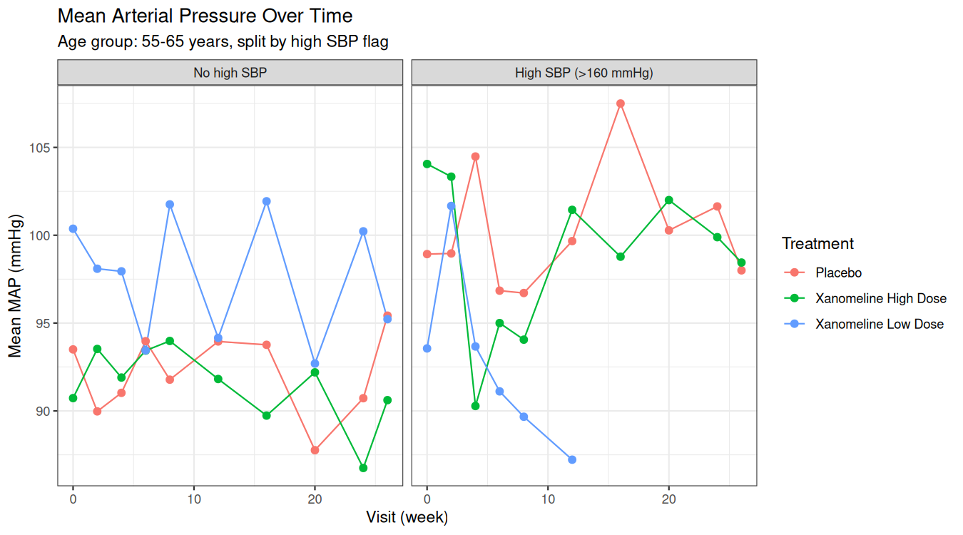
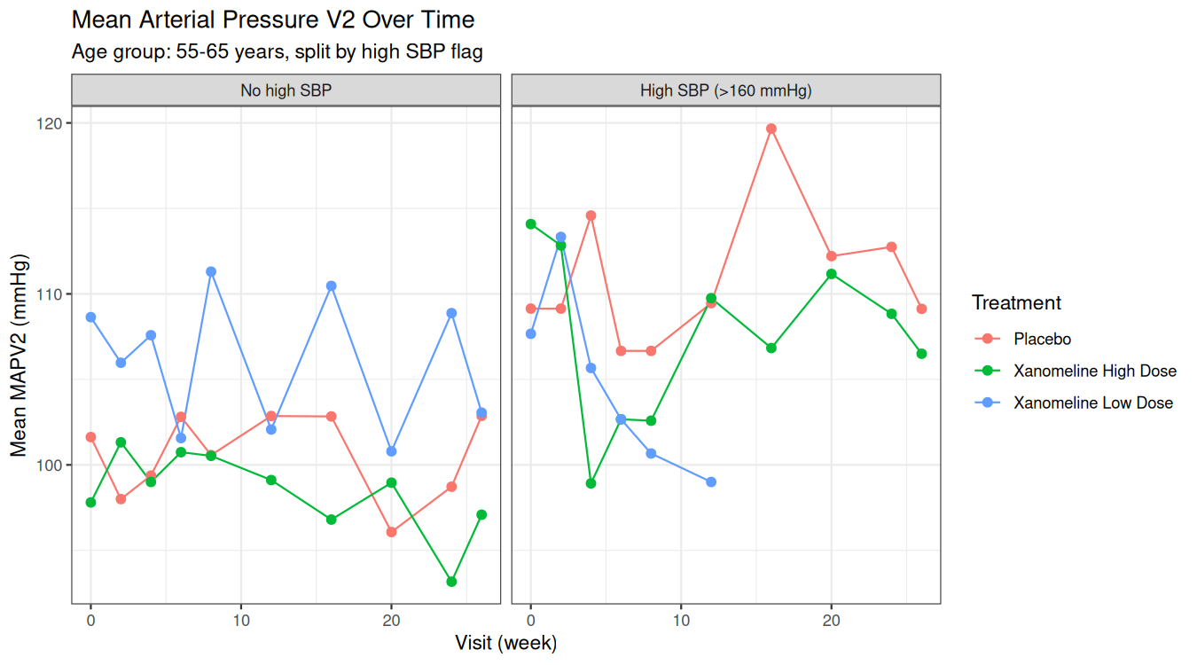
Task: Starting from templates/g_vs_map.R, create two plots of mean "MAP"/"MAPV2" over time (use visit number AVISITN), split by treatment arm (TRT01A) and restricted to patients aged 55-65. Optional: facet each plot into two, splitting by patients who have high systolic blood pressure (HISOBPFL == "Y") and those who do not (HISOBPFL == "N").

You’ll need to pre-process ADVS as follows first to compute the data points for the plot:

map_summary <- advs %>%
  filter(PARAMCD == "MAP" & AGEGR2 %in% c("55-65") & !is.na(AVISITN)) %>%
  group_by(AVISITN, AVISIT, TRT01A) %>%
  summarise(mean_aval = mean(AVAL, na.rm = TRUE), .groups = "drop")

Exercise 3: A Simple Visualisation

Solution:

ggplot(map_summary, aes(x = AVISITN, y = mean_aval, colour = TRTA, group = TRTA)) +
  geom_line() + geom_point(size = 2) +
  labs(
    title = "Mean Arterial Pressure Over Time",
    subtitle = "Age group: 55-65 years",
    x = "Visit (week)", 
    y = "Mean MAP (mmHg)", 
    colour = "Treatment"
  ) +
  theme_bw()

Repeat for PARAMCD == "MAPV2".

Exercise 3: Solution Plots

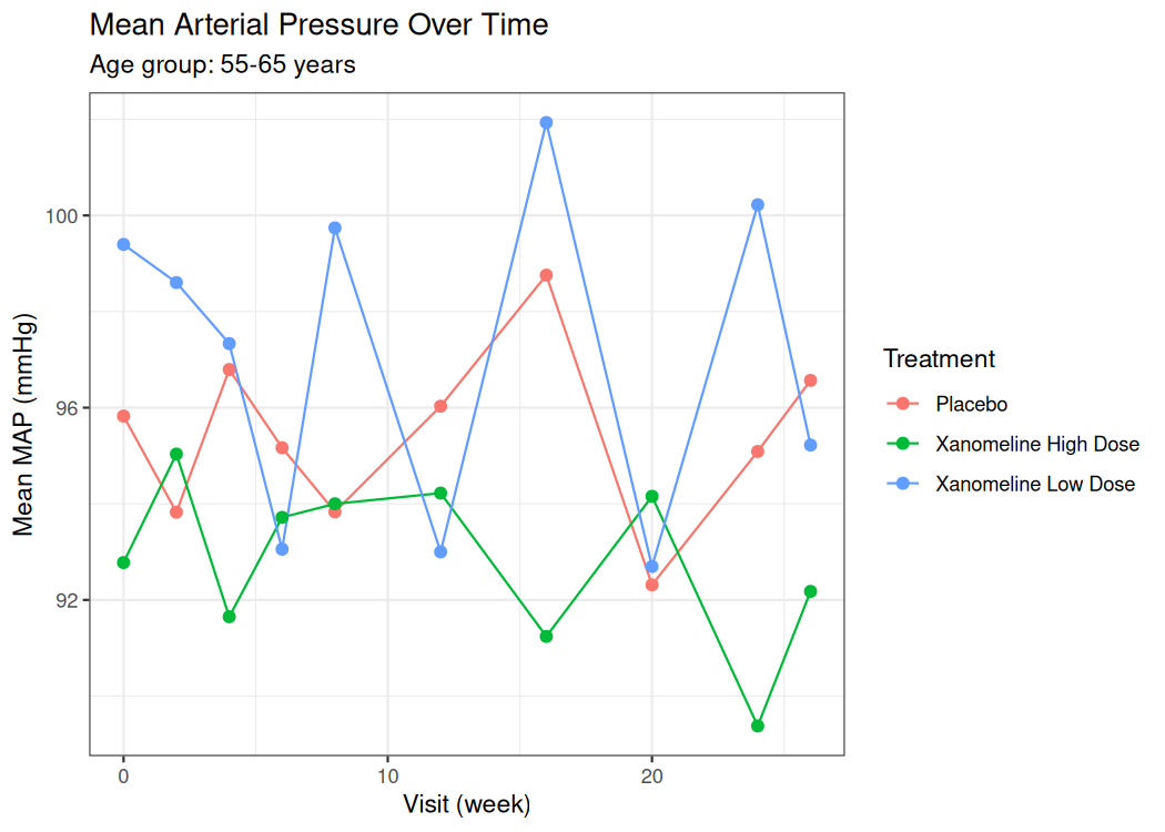
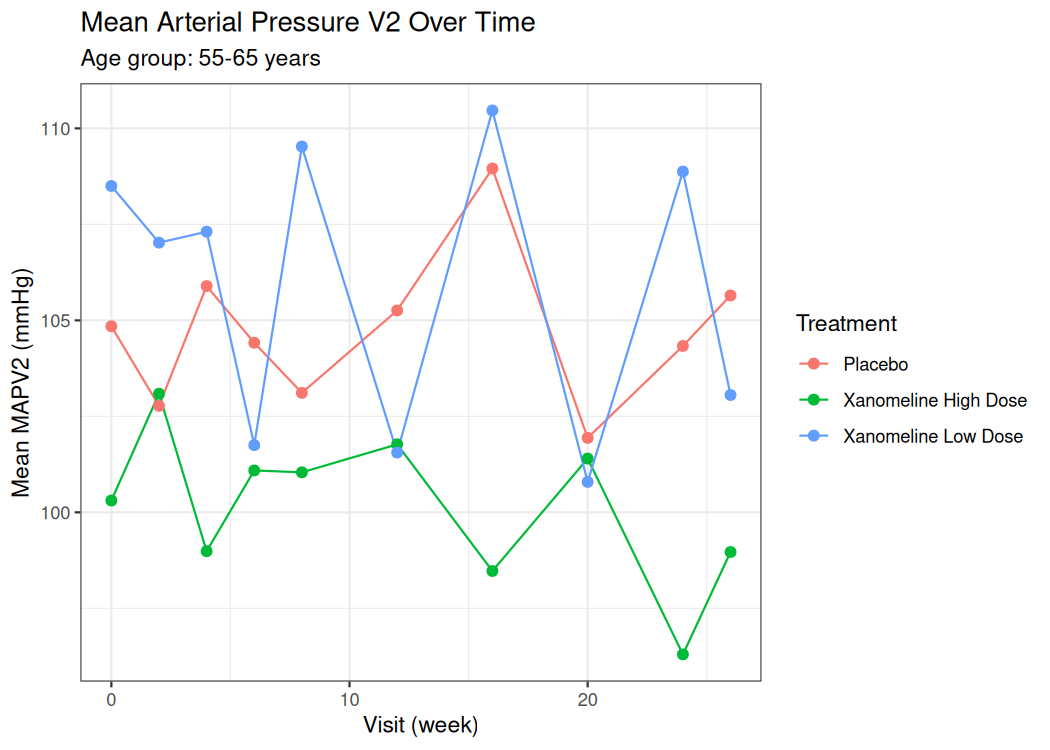
🤔Open question: How could you further enhance/improve these plots?

Exercise 3 (Optional): Faceted by `HISOBPFL`

Solution:

ggplot(map_summary, aes(x = AVISITN, y = mean_aval, colour = TRT01A, group = TRT01A)) +
  geom_line() + 
  geom_point(size = 2) +
  facet_wrap(~HISOBPFL) +
  labs(
    title = "Mean Arterial Pressure Over Time",
    subtitle = "Age group: 55-65 years, split by high SBP flag",
    x = "Visit (week)",
    y = "Mean MAP (mmHg)", 
    colour = "Treatment"
  ) +
  theme_bw()

Repeat for PARAMCD == "MAPV2". See solutions/solution_g_vs_map_faceted.R for the full solution.

Wrap-up

Summary and links for further reading

What we learned today:

The Clinical Data Pipeline (Raw → SDTM → ADaM → TLGs)…

Some pharmaverse packages that help support it

Examples of SDTM and ADaM datasets
- DM, VS, AE, EX
- ADSL, ADVS, ADAE

How to add variables to ADSL and parameters to ADVS to support analysis

How to use our datasets to generate a simple plot.

To go further:

Pharmaverse — https://pharmaverse.org/

More in-depth examples - https://pharmaverse.github.io/examples/

Thank You 🙏

Questions? Feedback?

Clinical Programming in R

About Me & This Workshop

Welcome!

Agenda

Background: The Clinical Trial Data Journey

The Clinical Trial Data Journey

1. Raw Data — Where it all begins!

2. SDTM — Standardising the data

SDTM in action: DM & EX

SDTM in action: AE & VS

3. ADaM — Analysis-ready datasets

ADaM in action: ADSL

ADaM in action: ADAE

ADaM in action: ADVS

4. TLGs — Answering questions!

TLG Example: AE Table

TLG Example: Pharmacokinetic Plot

Exercise Setup, Test Data & Packages

Exercise Setup and Test Data

Packages

Exercise 1: Working with ADSL

Exercise 1: Working with ADSL

Exercise 1a — New Age Group (AGEGR2)

Exercise 1a — New Age Group (AGEGR2)

Exercise 1b — High Systolic Blood Pressure Flag (HISOBPFL)

Exercise 1b — High Systolic Blood Pressure Flag (HISOBPFL)

Exercise 2: Working with ADVS

Exercise 2: Working with ADVS

Exercise 2: Working with ADVS

Exercise 2a — Derive MAPV2 (custom formula)

Exercise 2a — Derive MAPV2 (custom formula)

Exercise 3: A Simple Visualisation

Exercise 3: A Simple Visualisation

Exercise 3: A Simple Visualisation

Exercise 3: Solution Plots

Exercise 3 (Optional): Faceted by HISOBPFL

Wrap-up

Summary and links for further reading

Thank You 🙏

SDTM in action: `DM` & `EX`

SDTM in action: `AE` & `VS`

ADaM in action: `ADSL`

ADaM in action: `ADAE`

ADaM in action: `ADVS`

Exercise 1: Working with `ADSL`

Exercise 1: Working with `ADSL`

Exercise 1a — New Age Group (`AGEGR2`)

Exercise 1a — New Age Group (`AGEGR2`)

Exercise 1b — High Systolic Blood Pressure Flag (`HISOBPFL`)

Exercise 1b — High Systolic Blood Pressure Flag (`HISOBPFL`)

Exercise 2: Working with `ADVS`

Exercise 2: Working with `ADVS`

Exercise 2: Working with `ADVS`

Exercise 2a — Derive `MAPV2` (custom formula)

Exercise 2a — Derive `MAPV2` (custom formula)

Exercise 3 (Optional): Faceted by `HISOBPFL`